Highlight selected row in Excel

Certainly with large datasets, it can be an advantage to give the activated row (and possibly column) a different background color. Using Conditional formatting and a simple VBA script (macro) this is possible in Excel.

Conditional formatting

Let's start with the formula we are going to use for the conditional formatting.
The formula we are going to use to highlight the active row consists of two functions and is as follows:

=ROW()=CELL("row")

How the functions work

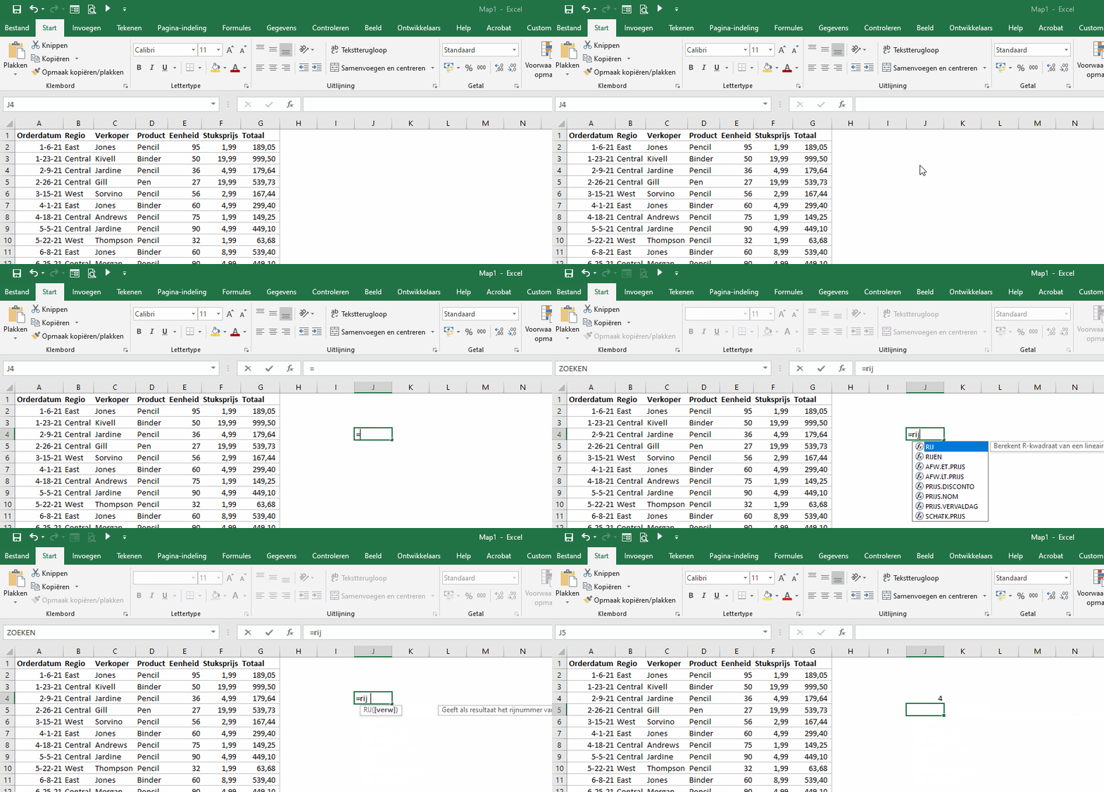
The ROW() function returns the row number of the cell in which the function was entered. If you enter the =ROW() function in cell J4, it will return 4 as a result.

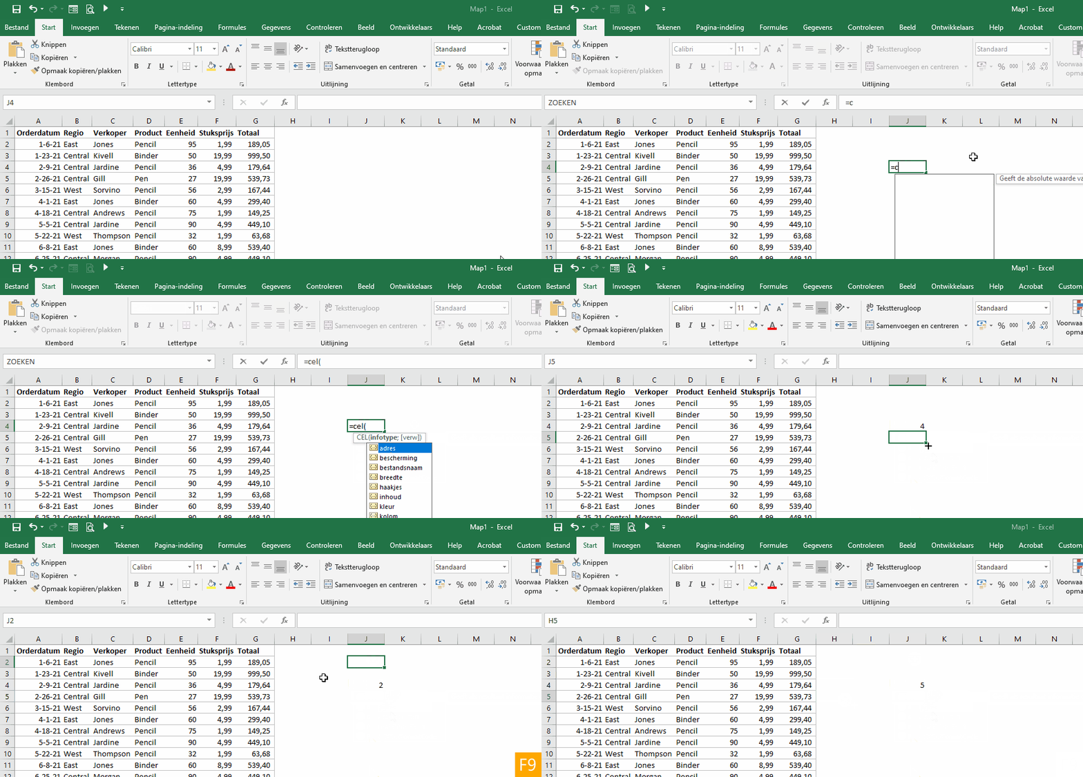
The CELL() function returns information about the formatting, content, or location of the selected cell. With this function you indicate in an argument what information you want to know about the selected cell. It will then be returned in the cell where you entered the function.

Selecting a cell and recalculating the formulas in your worksheet updates the value in the cell. You do this by pressing the function key F9 or navigating in the Ribbon menu to the tab FormulasCalculation and click Calculate now. Recalculates the formulas.

Explanation formula

If we above formula view there is the following. If the result of the ROW() function is the same as the result of the CELL("row") function, then the formula is TRUE. If the condition is not met, the result of the formula is FALSE.

If the result of the formula is TRUE, the background color of the row should be colored.

Formatting conditional formatting

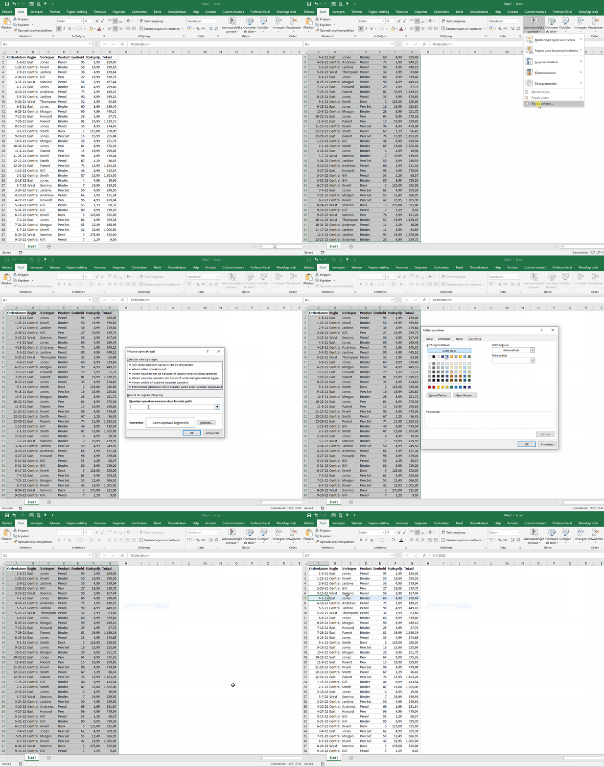
Select the range of your data table.

In the Ribbon menu go to StartStylesConditional formatting.

click on New rule….

A new window will open called New Formatting Rule.

Select the line Use a formula to control which cells are formatted.

Enter the following formula in the formula bar:

=ROW()=CELL("row")

Then click the button Opmaak.

A new window will open Format cells.

Go to the tab padding, select the desired background color and click OK.

After the window Format cells is closed, close the window New Formatting Rule by op OK to click.

Select a line in your data table and recalculate the formulas in your worksheet by pressing the function key F9 pressing or navigating to the tab FormulasCalculationCalculate now.

Create macro in the VBA editor

To have the formulas automatically recalculated after each selection change, we use a macro with the VBA editor.

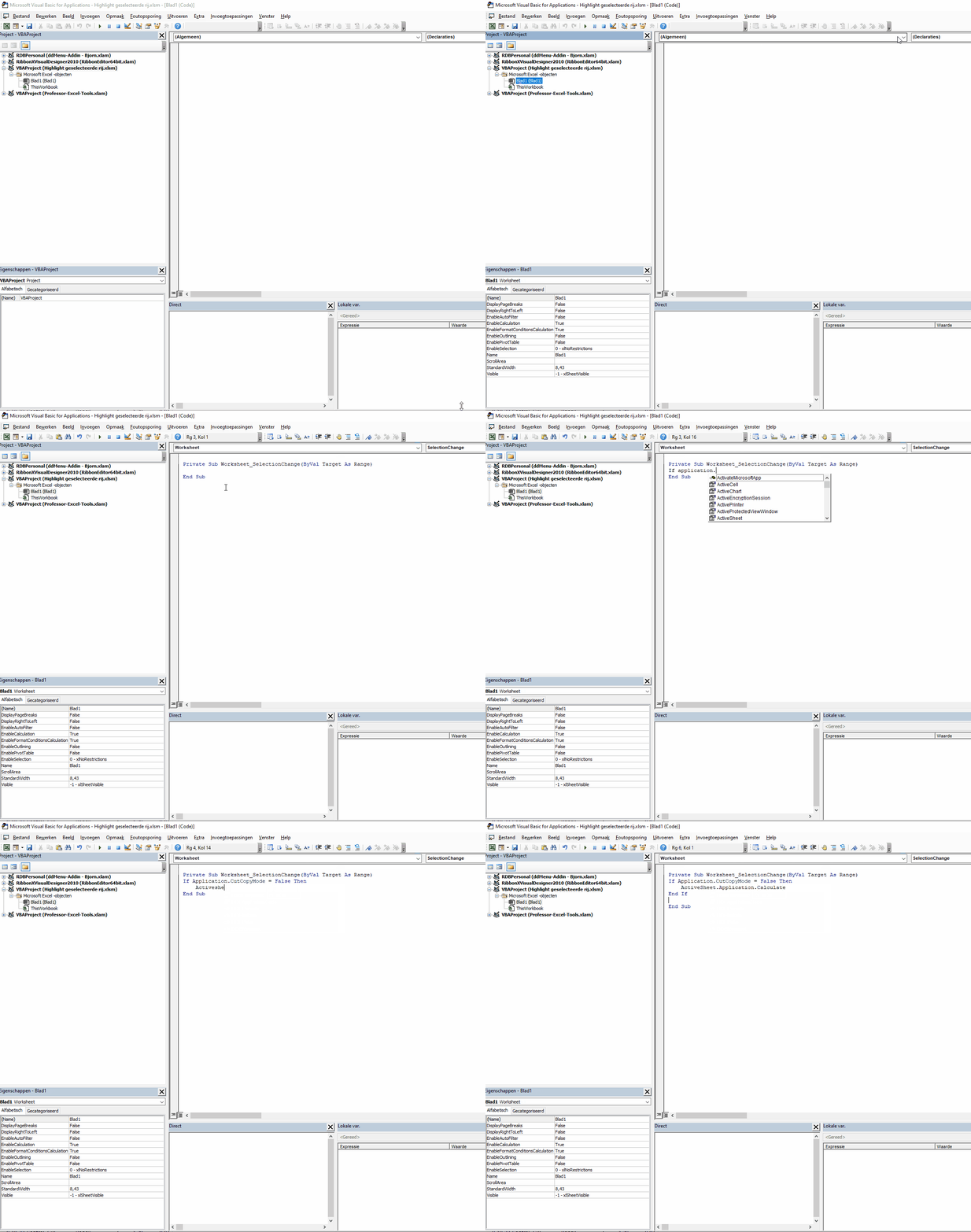
To open the VBA editor, press the function key Alt+F9. After which the VBA editor opens.

On the left side of your screen, select the sheet in which you have the conditional formatting.

Above the VBA editor, click the left drop-down menu and choose Worksheet.

A subroutine is automatically created called Worksheet_SelectionChange(ByVal Target As Range).

Enter the code below in the VBA editor:

Private Sub Worksheet_SelectionChange(ByVal Target As Range) If Application.CutCopyMode = False Then ActiveSheet.Application.Calculate End If End Sub

Close the VBA editor and select a few different lines in your data table to see if the VBA script works properly.

Save the file as an Excel workbook with macros.

Explanation of how VBA script works

With the IF statement we check whether values are being cut or pasted from the data table. If this is not the case, the formulas are updated by means of the code ActiveSheet.Application.Calculate.

If we don't apply the IF statement, it would not be possible to copy and paste values. Hence this piece of code.

Adjust background color of selected column

Do you (also) want to give the background of the selected column a different background color? Then enter the following formula in the conditional format:

=COLUMN()=CELL("column")

Downloads

If you can't figure it out with the above guide alone, download the sample file or ask a question by leaving a message.