Create Dynamic Range in Excel

Dynamic range with formulas

For the sake of convenience, in this example, we will assume a customer base. We can assume that there are regular changes here. If things go well, new customers will be added regularly.

You can select the relevant debtor via a drop-down list, after which all other details are entered.

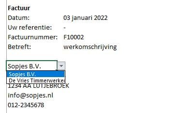
Create drop-down list

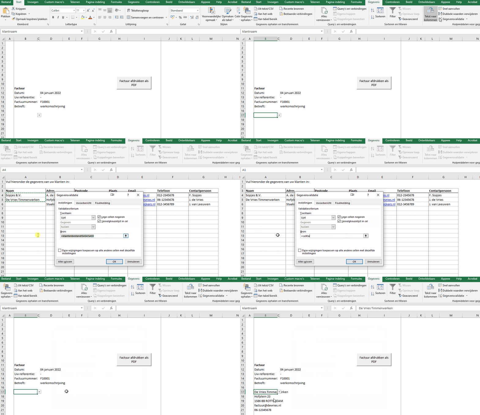
To create a drop-down list, select the cell in which you want the list to appear (for example, B17). In the ribbon, go to the tab Facts the group Data Tools and click Data Validation. A new window will open.
under the tab Settings choose you at To allow: for “List” and at Source: enter the range (see image below).

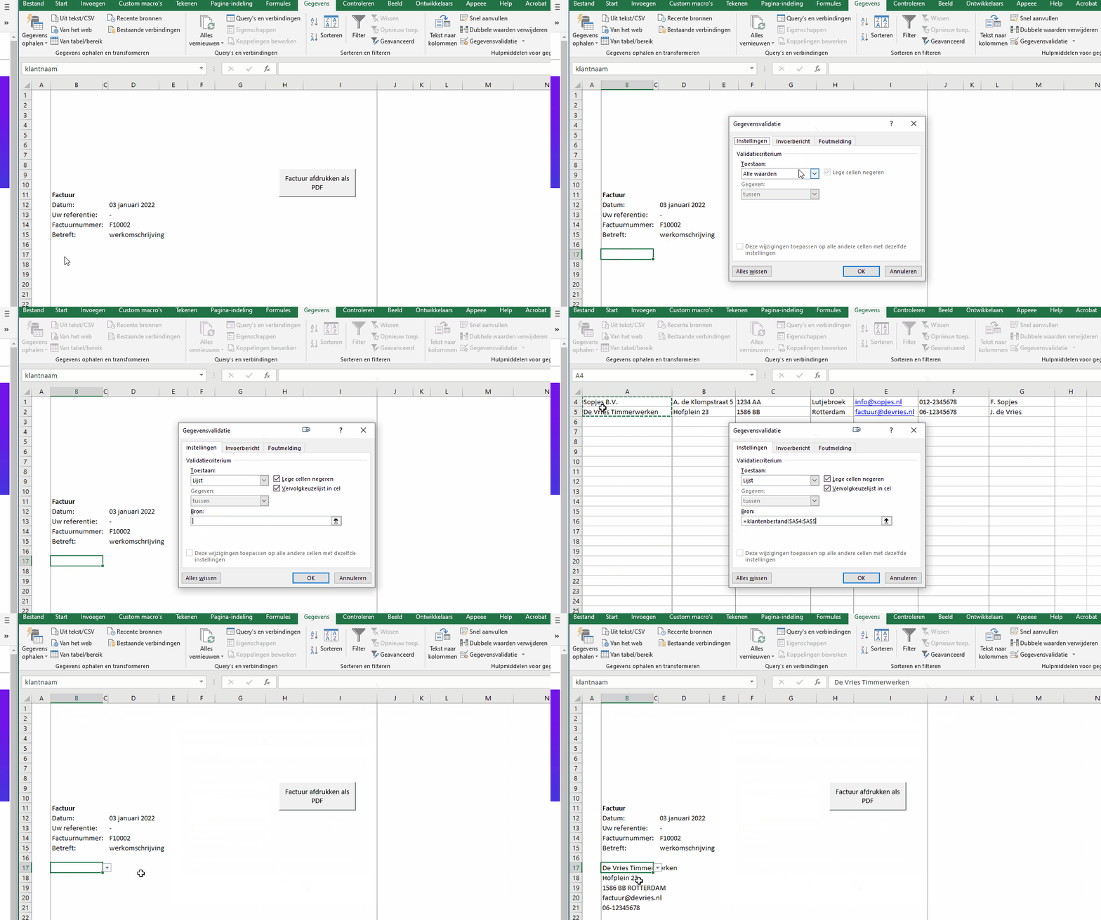
Every time you add a customer to the customer database, the scope of the drop-down list must be adjusted. This is not desirable. The best thing would be if this were a dynamic range. Below you will find an explanation of how we are going to do this.

Make range dynamic

In the formula I use the functions: OFFSET and COUNTA. The OFFSET function works as follows: OFFSET(ref, rows, columns, [height], [width]).

The argument refer can be seen as a beacon. You indicate here from which cell you want to perform the shift. In the example, this is cell A3. From this cell we want to shift

Rows indicates how many rows you have from refer want to move up or down. In the example we start in cell A3. This cell contains the description of the relevant column. We do not want these displayed in the drop-down list. We therefore move down one row, so enter a 1 here. If you enter a negative number, you move up.

Columns indicates how many columns you have from refer to move left or right. Because we remain in the same column, we enter a 0 here.

With the last two arguments, we set the height and width of the dynamic range. To determine the height of the range we use the function NUMBER. This function counts the number of non-blank cells.

The function NUMBER is put together as follows: COUNTA(value1, [value2;...]). For value1 we fill in column A:A after which all non-empty cells in this column are counted. We then subtract 2 from this because the values in cells A1 and A3 do not count.

The final formula is then as follows: =OFFSET(customer base!$A$3;1;0;COUNTA(customer base!$A:$A)-2;1).

Manage names

We can enter the above formula at the source of the drop-down list, but we can also save the formula in an easier-to-remember name. You do this with the option Define name.

In the ribbon, go to the Formulas tab the group Defined Names and click Define name.

A new window will open called New name.

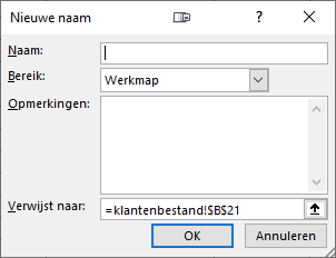
Fill in the input field Name: an easy-to-remember name for your formula.

at the field Refers to: do you enter the formula =OFFSET(customer base!$A$3;1;0;COUNTA(customer base!$A:$A)-2;1) in.

Then click on OK and the defined name is saved.

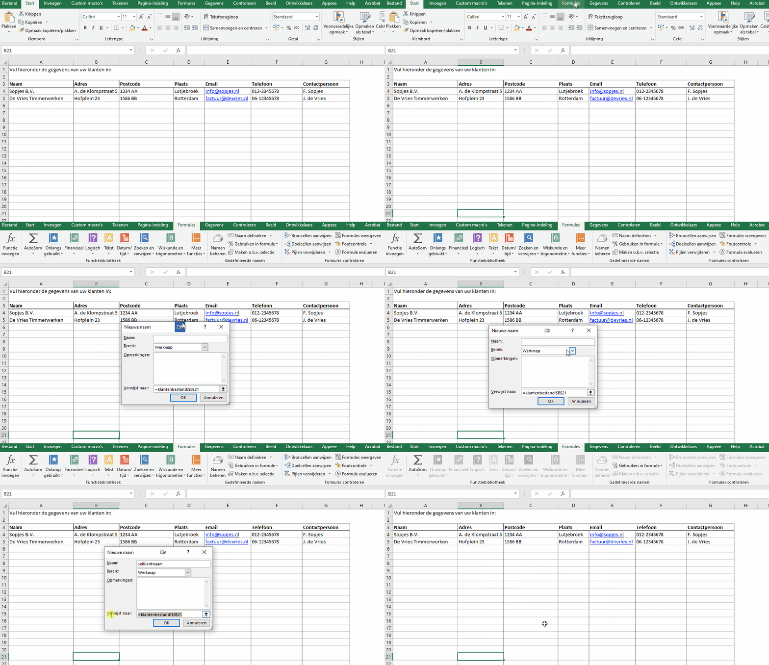
Make preset list dynamic

Only now the reference of the drop-down list by changing the reference to =selCustomer name. click on OK to save the dynamic drop-down list.

Forgot the name of the named range? Select the input field Source: and press the F3 function key. A new window will open with all named ranges. This also prevents the chance of typos.

If you now add a new customer to the customer database, it will automatically be added to the drop-down list.